Sentiment Analysis of the 20th Bundestag legislative period

Recently, I found out about Bundestag Open Data - basically all the neat bureaucracy of Bundestag is digitalized and for the more recent legislative periods actually very nicely formatted and well-documented. On the website they say this data is open for usage by interested users. With Bundestag elections approaching, why not analyze this masterpiece of governmental transparency.
First of all, the results of this analysis probably have much noise in them. I suppose the methods of analysis used here are neither reliable in any way, nor applied professionally. This project is not intended to portray any political party in a better or worse light but was undertaken out of curiosity and to explore data analysis and natural language processing.

Data Preparation

Data Sources

So what kind of data do we have? The Bundestag DIP (Dokumentations- und Informationssystem für Parlamentsmaterialien) provides a well-documented API, allowing queries for various types of parliamentary data, such as members of Bundestag, procedural details, and voting records. While the dataset is extensive, the focus is on the Plenarsitzungen (plenary sessions), where parliamentary debates and speeches occur.

Each Plenarsitzung is transcribed in a highly detailed protocol, capturing literally every spoken word, including interruptions and interjections. Although the API provides links to these protocols in PDF format, parsing PDFs for automated text extraction, especially for isolating individual speeches, is quite cumbersome. Fortunately, more recent protocols are also available as structured XML files with super nice documentation. These XML files have been used consistently since the 19th legislative period, though they somehow also work for the 18th period. In total, 696 protocols spanning three legislative periods were available.

Exploring the Data

The metadata for each protocol includes the following structure:

<kopfdaten>
    <plenarprotokoll-nummer>Plenarprotokoll <wahlperiode>20</wahlperiode>/<sitzungsnr>211</sitzungsnr></plenarprotokoll-nummer>
    <herausgeber>Deutscher Bundestag</herausgeber>
    <berichtart>Stenografischer Bericht</berichtart>
    <sitzungstitel><sitzungsnr>211</sitzungsnr>. Sitzung</sitzungstitel>
    <veranstaltungsdaten><ort>Berlin</ort>, <datum date="31.01.2025">Freitag, den 31. Januar 2025</datum></veranstaltungsdaten>
</kopfdaten>

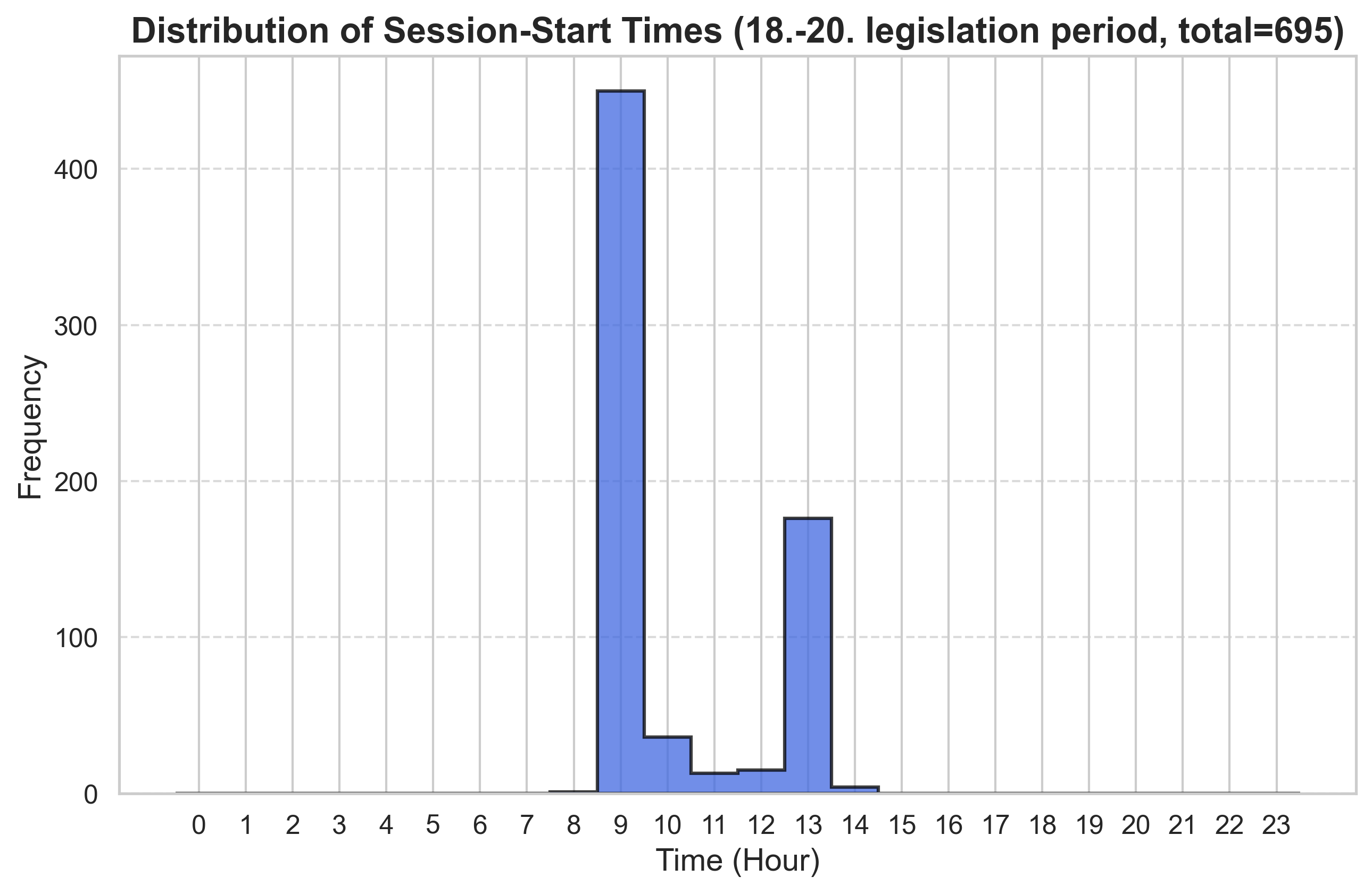
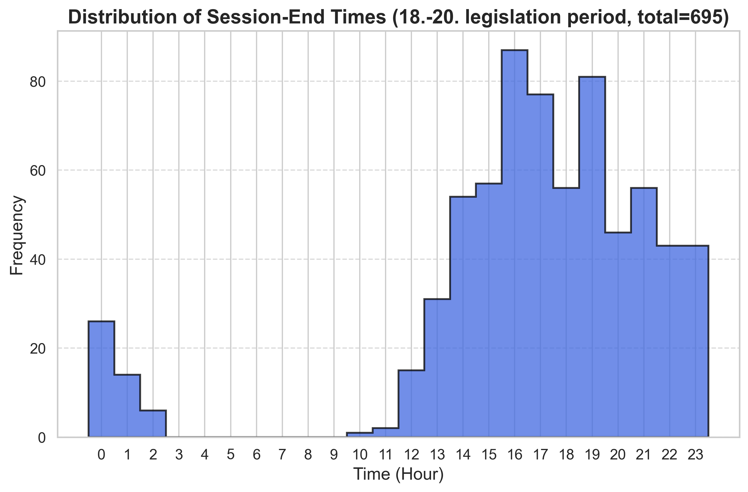
From this metadata, we can extract session start and end times, track speech frequency per party and legislative period, and analyze other temporal aspects of parliamentary activity. The following time-frequency plots illustrate the distribution of session start and end times (total: 696 sessions):

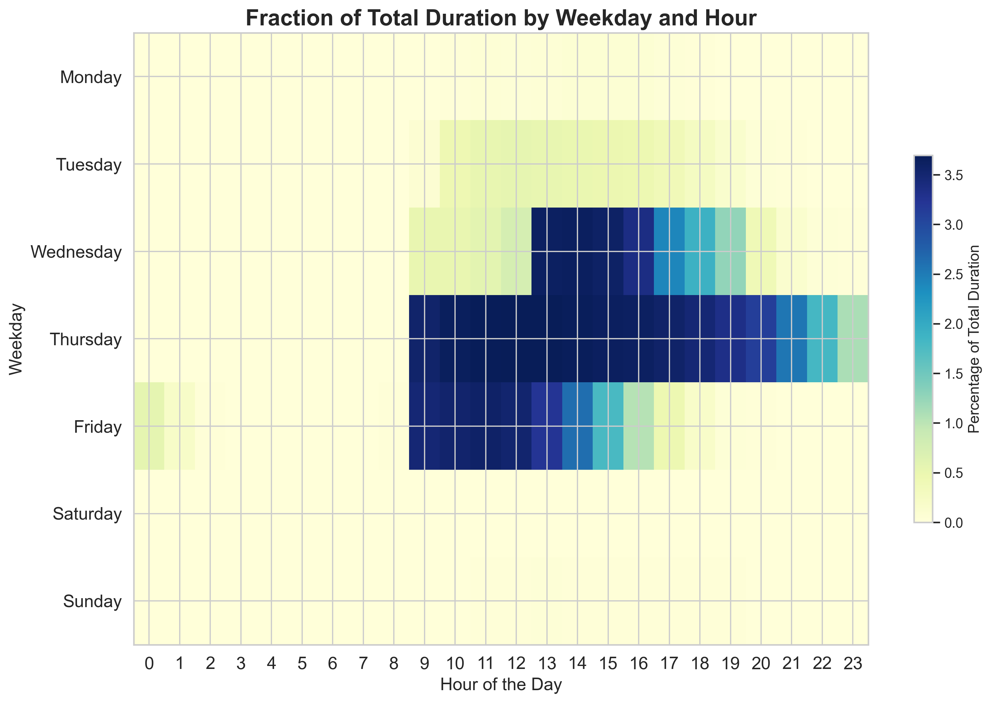
So they are actually working quite long. Or one could basically sum for each weekday and hour the total time, which was spent in a session (i.e. if a session was starting at 11:20 and ended at 15:20 on a wednesday, we add 40 minutes to wed/11, 60 minutes to wed/12, … and 20 minutes to wed/15), then we could consider the fraction of the sum of all time spent in session, which gives some kind of distribution over the weekday/time combinations. We obtain:

ChatGPT agrees exactly with what we can observe in the plot:

“> On which weekdays do plenary sessions occur?”

Plenary sessions in the German Bundestag typically take place from Wednesday to Friday during sitting weeks.

• Wednesday: Often starts in the afternoon.
• Thursday: Usually the main day for key debates.
• Friday: Often concludes earlier than other days.

There are many more things one can analyze here, for example the change of the duration of sessions over a legislative period and so on. However, our primary focus is on analyzing the speeches themselves.

Speech Extraction

The first step towards the analysis of the actual speeches therefore consisted of the extraction of the relevant data from the xml documents. For the sake of computation time and because one can hypothesize that the sentiment in the speeches strongly plays together with which parties are forming the government¹, so it is reasonable to only go for the 20th period as a first approach. There were 211 Plenarsitzungen in the 20th legislative period of Bundestag. One can easily extract all the speeches and the person giving the speech with the corresponding ID (every member of Bundestag has an ID, which can also be used later to query the data for that specific person). Essentially, we now have data of the following form

Index	Speech ID	Person ID	Session ID	Party	Speech Text	Date
0	ID2020900100	11003231	20209	NaN	Frau Präsidentin! Liebe Kolleginnen und Kollegen…	29.01.2025
1	ID2020900200	11002735	20209	CDU/CSU	Frau Präsidentin! Liebe Kolleginnen und Kollegen…	29.01.2025
…	…	…	…	…	…	…
26392	ID2020409700	11005249	20204	SPD	Vielen Dank. – Frau Präsidentin! Werte Kolleginnen und Kollegen…	06.12.2024
26393	ID2020409800	11004288	20204	Die Linke	Ich will es unumwunden sagen: Die Linke kann das…	06.12.2024

Total: 26394 speeches (only considering 20th legislative period).

Potential problems and impurities

As one can see above, in some cases the group/party for the speech couldn’t be extracted (in roughly 3460 cases), this is because for the speeches by members of the current government, they don’t provide the group/party directly in the metadata of the speech - they only provide the current role like Bundeskanzler. However, we can still obtain the group/party for these speakers, by using the person’s id.

Apart from the fact that the group/party was formatted poorly in some cases, there was some member of the parliament who was apparently part of SPDCDU/CSU which was kind of ambiguous. I have no idea what happened there, but it was just a member of CDU.

Additionally, there are some speeches which are not by members of the parliament, their IDs can be distinguished (using the documentation). Some of them still have a party others not, those who could not be identified with a party are removed from the dataset (around 818).

However, there might be another problem. It might be questionable, why there are so many speeches. Well, it turns out that in Government Q&A sessions (it’s probably not called like that), every question and answer is counted as a speech on its own. One can argue that this is still relevant data. After dropping all the speeches which were shorter than 40 chars, the dataset is more or less cleaned and contains a total of 25560 speeches.

Data Analysis

Simply counting the speeches per party/group yields the following:

Party/Group	Number of Speeches
SPD	6078
CDU/CSU	5760
B90/DIE GRÜNEN	4515
FDP	3665
AFD	3034
DIE LINKE	1873
FRAKTIONSLOS	488
BSW	147

We now want to employ different strategies to analyze the sentiment in these different speeches. The most standard approach to sentiment analysis is text classification, i.e. using models which label the given text as positive/neutral/negative. The obvious problem when applying these models to our speeches is, apart from the fact that the lengths of the speeches exceed the token limit of some models, the granularity. Obtaining one prediction of exactly one label for a huge speech isn’t very descriptive and definitely not sufficient for our purposes. I suppose there are only a handful of speeches which would be labeled “positive”, as the overall tone of political debates naturally contains more negative language. So it is reasonable to split the texts into smaller chunks (for example simply in sentences) and then perform these analyses on these smaller chunks.

Natural Language Processing

A useful library also for other purposes in the field of natural language processing is spacy. Running the spacy pipeline, we also obtain all the tokens and their lemmatizations (which will also be useful in the following). There is actually much more possible here, one could for example also consider spacy’s named entity recognition and entity linking, however, we will keep it simple. To not blow up the size of the data here, we only store really necessary things like the lemmatizations and the sentences - this is kind of wasteful, because if we decide later that we also want to analyze different things which are obtained from spacy’s NLP functionality we would need to recompute, however we won’t. It already takes about 1h to apply this processing to the speeches of the 20th legislative period (making use of maximal spacy’s pipeline and also maximal parallelization on Macbook M1, 2020).

To illustrate what we got from this step, consider thee following:

"Frau Präsidentin! Liebe Kolleginnen und Kollegen! Diese Debatte heute hat eine große Bedeutung, ..."

Extraction of sentences gives:

['Frau Präsidentin!', 'Liebe Kolleginnen und Kollegen!', 'Diese Debatte heute hat eine große Bedeutung, [...]', .... ]

Lemmatization yields:

[('Frau', 'Frau'), ('Präsidentin', 'Präsidentin'), ('!', '--'), ('Liebe', 'lieb'), ('Kolleginnen', 'Kollegin'), ('und', 'und'), ('Kollegen', 'Kollege'), ('!', '--'), ('Diese', 'dieser'), ('Debatte', 'Debatte'), ('heute', 'heute'), ('hat', 'haben'), ('eine', 'ein'), ('große', 'groß'), ('Bedeutung', 'Bedeutung'), (',', '--'), ...]

Berlin Affective Words List

The first and probably most intuitive thing one could do with the speeches is to simply use a list of words of which we know that they are more likely to have a negative/positive connotation and numerically quantify this, using some score and then simply average these scores for each text. Obviously, there are already things like these for the German Language. One example is the Berlin Affective Words List (BAWL-R):

The Berlin Affective Word List - Reloaded (BAWL-R) is a German database containing normative ratings for emotional valence, emotional arousal, and imageability for more than 2,900 German words.

One possible problem is that this list is from 2009, but I suppose a language cannot change too much in its semantics over this time. Though there might be commonly used words which simply aren’t part of this list. These possible inaccuracies have to be kept in mind when thinking about the results.

I have no idea if these measurements are properly psycho-linguistically justified, but the dataset seems quite useful (for a more sophisticated description, check out these nice papers by Melissa L. H. Võ et al.: doi:10.3758/BRM.41.2.534, doi:10.3758/BF03193892). It’s basically a big table of the following form

WORD	WORD_LOWER	WORD_CLASS	EMO_MEAN	EMO_STD	AROUSAL_MEAN	AROUSAL_STD	IMAGE_MEAN	IMAGE_STD	LETTERS	PHONEMES	SYLLABLES	Ftot/1MIL	N	FN	HFN	FHFN	BIGmean(TOKEN)	ACCENT
AAL	aal	N	-0.5	0.707107	2.380952	1.244033	6.555556	0.726483	3	2.0	1	13.333333	6	3182.00	3	3175.17	83677.500000	1.0
AAS	aas	N	-2.1	1.100505	2.631579	1.422460	5.444444	0.881917	3	2.0	1	1.000000	6	10568.83	5	10568.50	30120.500000	1.0
ABART	abart	N	-1.6	0.699206	3.277778	1.017815	2.333333	1.322876	5	5.0	2	1.166667	2	3.00	1	2.33	80270.000000	1.0
ABBAU	abbau	N	-1.0	1.169795	3.000000	1.297771	2.227273	1.231794	5	4.0	2	14.500000	1	6.83	0	0.00	94054.750000	1.0
ABBAUEN	abbauen	V	-0.8	0.920000	2.105263	1.242521	3.670000	1.580000	7	6.0	3	15.500000	3	51.00	1	38.00	238806.333333	1.0
…

The three interesting features we get from this table are:

• EMO_MEAN (emotional valence mean) - this is basically just the mean over different uses of the word ranging from pleasant to unpleasant. The highest value is 2.9 for the word Liebe and the lowest value is -3.0 for the word Giftgas.

• AROUSAL_MEAN (emotional arousal mean) - this ranges from calm to excited. The highest value is 4.7 for Attentat and the lowest value is 1.1 for Schlaf.

• IMAGE_MEAN (imageability mean) - Wikipedia: Imageability is a measure of how easily a physical object, word, or environment will evoke a clear mental image in the mind of any person observing it. The highest value here is 6.9 for words like Klee and Mond

For each of these fields, there is also the corresponding standard deviation. For example, for emotional valence words with high standard deviations tend to vary a lot in their use as positivity and negativity in different contexts.

The approach is now to simply take the lemmatizations of a speech and compute the averages for these values. The obvious problem is that the context is disregarded completely. The context could be extremely relevant in cases like irony or similar. The hope is, that this approach still yields some kind of measure for the kind of tone of a speech, especially when averaging over all speeches by a party/group.

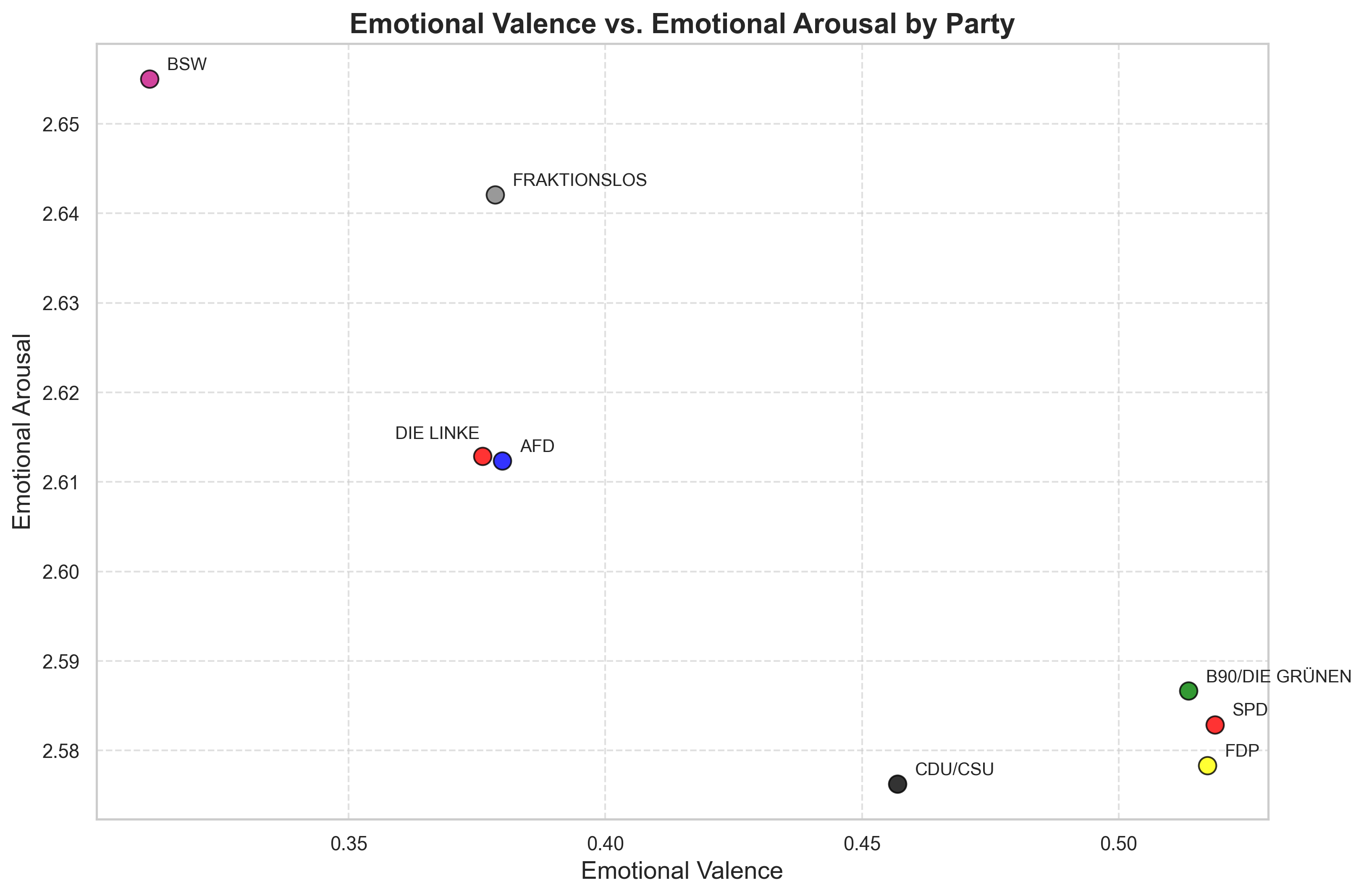
Grouped by party, we can get the following (20th legislative period):

Party/Group	avg. emotional valence	avg. emotional arousal	avg. imageability
BSW	0.311232	2.655031	3.756075
DIE LINKE	0.376087	2.612857	3.688495
FRAKTIONSLOS	0.378566	2.642078	3.798500
AFD	0.379939	2.612371	3.740115
CDU/CSU	0.456902	2.576281	3.654246
B90/DIE GRÜNEN	0.513605	2.586667	3.648534
FDP	0.517266	2.578349	3.617487
SPD	0.518748	2.582901	3.623795

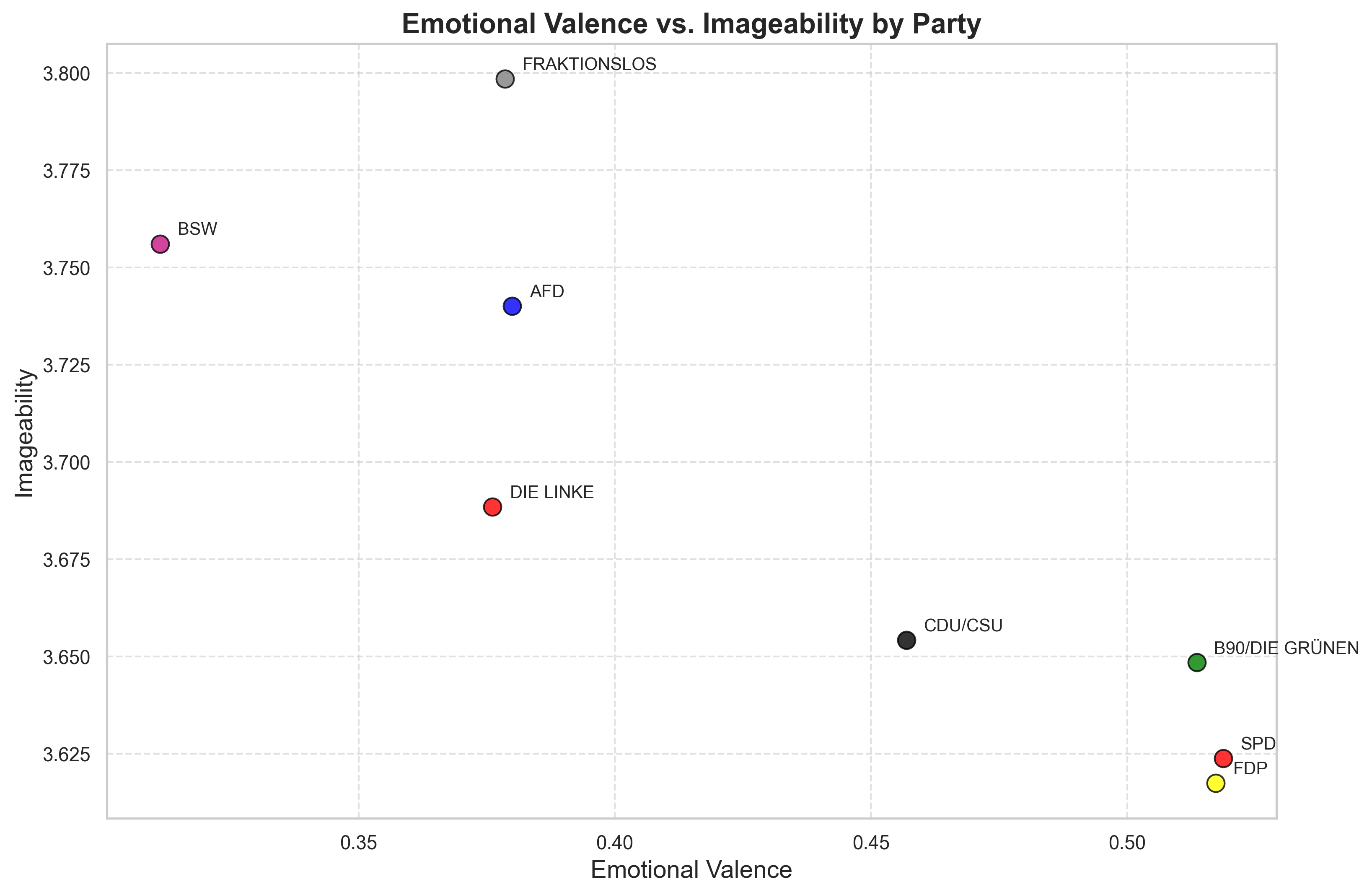
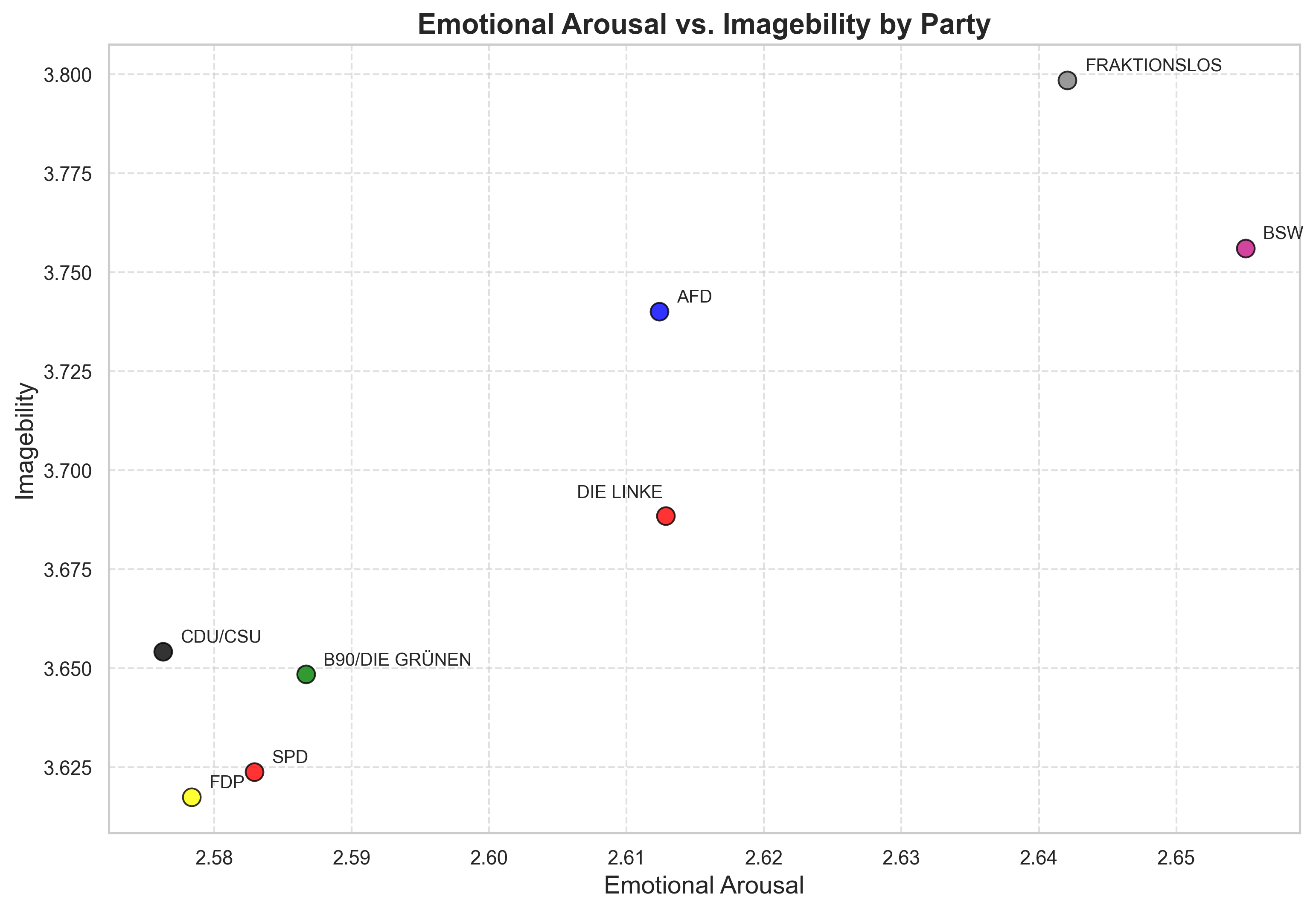
What’s quite interesting here is, that one can observe a higher emotional valence for the government parties (B90/DIE GRÜNEN, SPD, FDP).

To make it more apparent consider the following plots, we stick to two dimensions to increase visibility:

The overall differences in average imageability and arousal are rather tiny and it is questionable in what sense this is really significant. Additionally, one has to keep in mind that the number of speeches varies across the parties. Also, these plots do not indicate any similarity in the topics or anything else, but only in the scores in the different parameters of the words which are used. It is open whether a higher or lower emotional valence is good or bad. The interpretation of the plots is left to the reader. I think it is also important to talk about topics which have a rather negative connotation. The most interesting thing one can observe here is the cluster of the government parties.

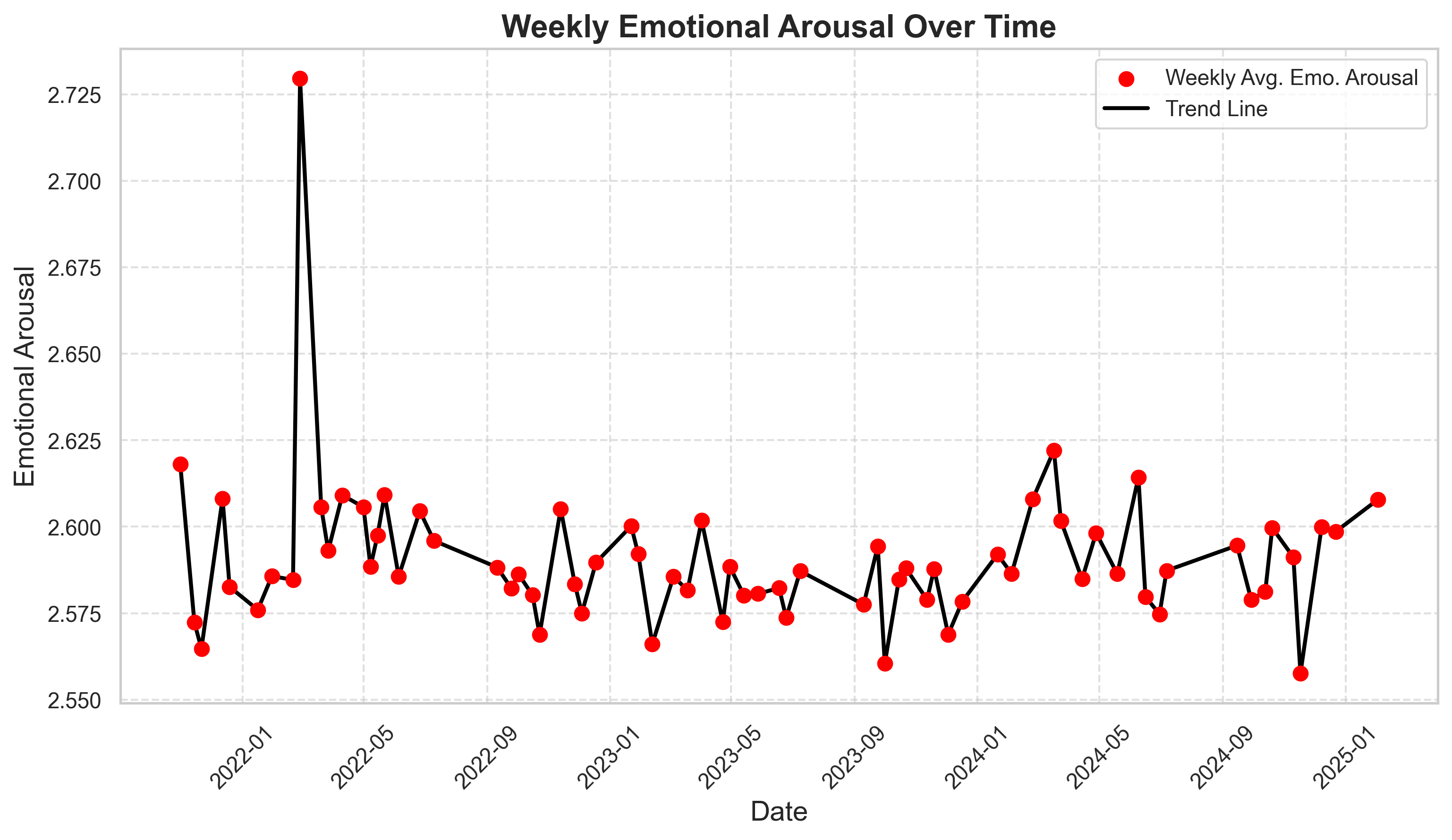
Another interesthing thing which was observable when plotting the emotional arousal over time, is a big peak in February 2022 which is probably because of the start of Russia’s invasion of Ukraine:

Transformer

The obvious problem of the approach above is that it fails to capture any notion of the contexts of words. One of the main ideas was to use some kind of transformer. This was also the motivation for splitting the speeches into sentences in the first place. A transformer is simply a special type of Neural Network or Machine Learning Architecture (which is the T in GPT). Many pretrained language sentiment analysis models can for example be found on https://huggingface.co/. Most of these models simply classify a sequence of tokens as 'positive', 'neutral', 'negative' with a corresponding probability (i.e. we obtain 3 floating point values, let these be $p_+, p_\circ, p_-$). We could then for example compute a score as $s = p_+ - p_-$, and the average over these scores for each sentence.

The first model we can use is called germansentiment. It is described in the paper Training a Broad-Coverage German Sentiment Classification Model for Dialog Systems (Oliver Guhr et al.) and is using Google’s BERT architecture.

After roughly 7 hours of computation (processing of all the sentences), we obtain the following results:

Party/Group	Mean Score	Standard Deviation	# speeches
DIE LINKE	-0.075661	0.007013	1844
AFD	-0.075288	0.006991	2989
FRAKTIONSLOS	-0.070809	0.010466	482
CDU/CSU	-0.060228	0.006375	5670
BSW	-0.059981	0.008759	139
B90/DIE GRÜNEN	-0.045689	0.008512	4454
SPD	-0.042663	0.007425	5975
FDP	-0.036108	0.007429	3619

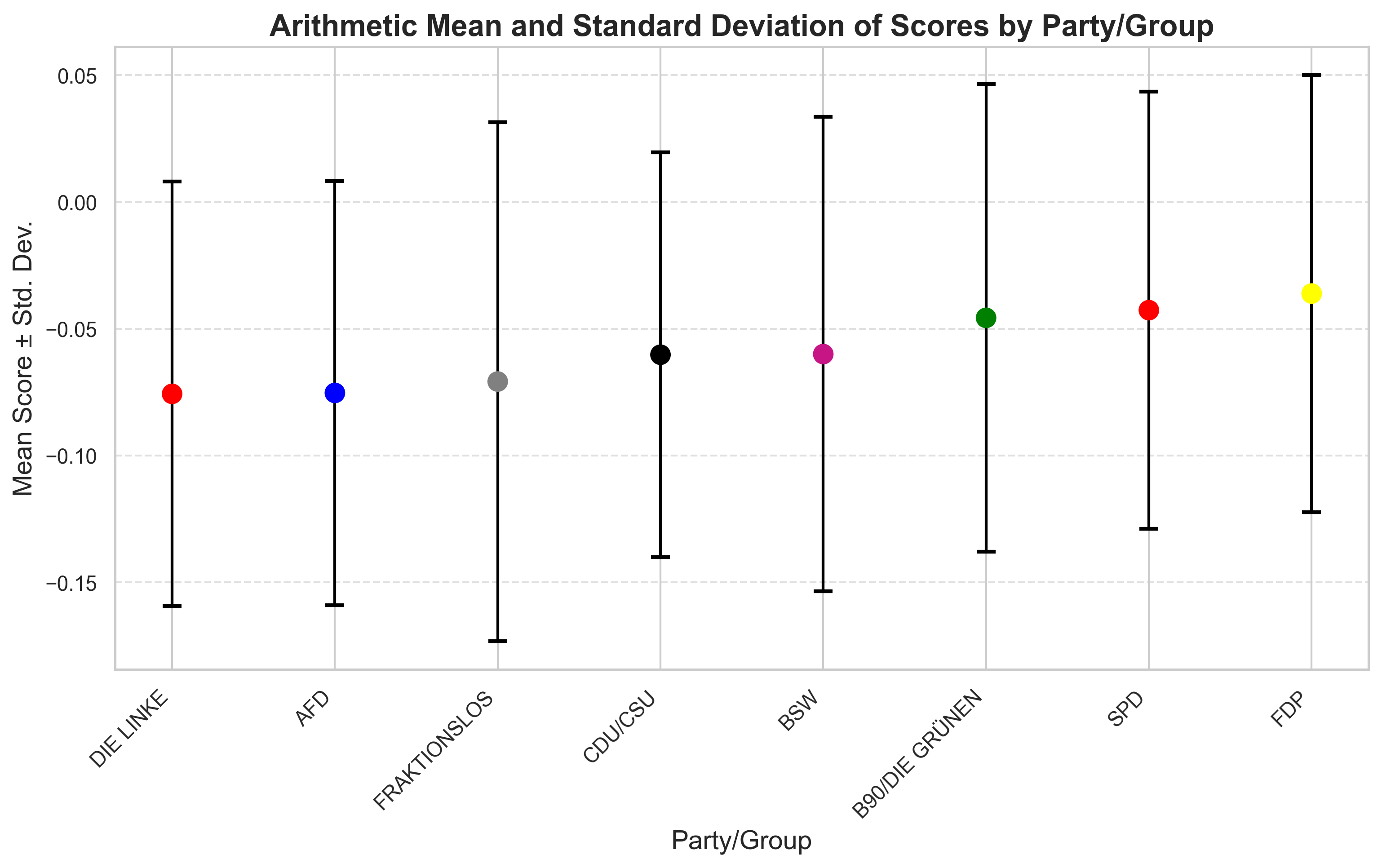
We additionally compute the standard deviation over the speeches (i.e. we first compute the scores of each speech, by averaging and then computing the average over all speeches and the variance over all speeches, while grouping by party)

What’s interesting here is that we again have the government parties with a more positive score. While the arithmetic means give some insights, it is important to make sure that this is not just the random result of very noisy data, which it might actually be, considering the following plot (which depicts the standard deviation):

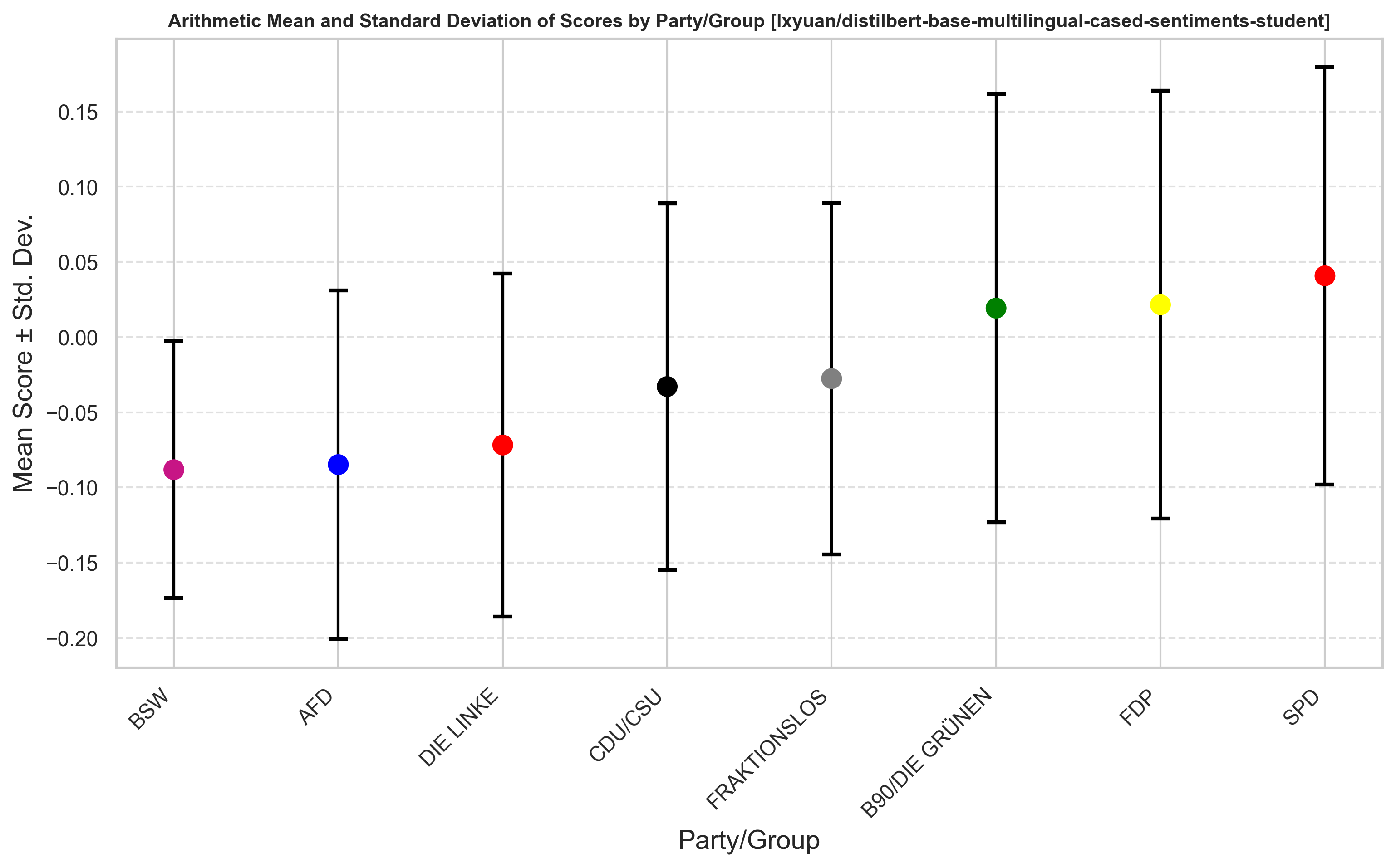
The hope is to maybe validate the results or get more robust results by applying a different model: lxyuan/distilbert-base-multilingual-cased-sentiments-student, which supports multilingual sentiment analysis with the same labeling and is quite popular. It is also based on Google’s BERT architecture. The results after 3 hours of processing are the following:

Party/Group	Mean Score	Standard Deviation
BSW	-0.088206	0.085423
AFD	-0.084820	0.115808
DIE LINKE	-0.071799	0.114041
CDU/CSU	-0.032914	0.122025
FRAKTIONSLOS	-0.027618	0.116882
B90/DIE GRÜNEN	0.019227	0.142499
FDP	0.021513	0.142258
SPD	0.040736	0.138806

Clearly, the whole score is much more spread here. Interestingly, it is again the case that the three government parties obtain higher scores than the opposition, while the general order among other parties is not reproducible.

Applying the same visualizations as before:

Things to do

Obviously, one could do so much more here, the next interesting thing, which would probably yield much better and interesting multidimensional results would be the zero-shot classifier using something like OpenAI API. Some ideas:

1. Do more standard data analysis.
   1. Different features for specific members of Bundestag
   2. Extract the comments from the protocols and analyze them for different parties
   3. Use more historical data
2. Improve sentiment analysis
   1. Zero-Shot LLM classification (this would have been the way to go) We can choose a multitude of labels and use the popular approach of zero-shot classification (provide the LLM with the speech and the labels and ask it to classify, e.g. Open AI API) - first of all, doing this is probably even much more precise than the classification using these small transformers, additionally, we can use many labels for different aspects of the speech like: Policy Areas, Political Strategy and Intent, Rhetorical Style and Tone, Values and Ideologies or Audience and Target Groups. I might do this for comparing the new legislative period with the previous one if I find time - I think this approach is also much more convenient, because we simply have to do API calls :).
   2. Train own model
   3. Train a prediction model (predicting the party based on the speech)